


This year, 2019, commemorates the 50th anniversary of one of humanity’s most incredible achievements thus far: of people physically reaching the Moon. On July 20, 1969, Apollo 11 landed on the natural satellite and broadcast a live view of the lunar surface, Earth, space and of astronauts working on the surface.
Yet still, there are doubts these days that humans actually achieved this feat. For example, the following question appeared on Quora on August 23, 2018: “When will the existence of the Van Allen belt and our inability to penetrate its harsh radiation with today’s technology force NASA to admit it faked the moon landing?”
What surrounds Earth?
Some people believe we never went to the Moon because of the existence of the Van Allen radiation belts. The idea is that any astronauts en route to outer space has to pass through these belts and, in so doing, they would receive a lethal dose of radiation.
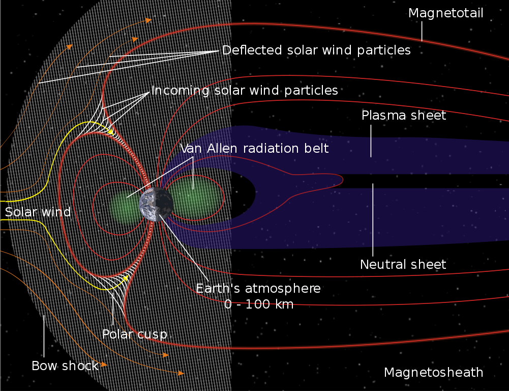
These belts are the result of Earth’s magnetic field working like a magnetic trap – or an accelerator – confining the particles of the solar (mostly) wind, and sometimes accelerating them on their orbits within the belts to nearly the speed of light.
These belts are shaped like two nested doughnuts. Their sizes change depending on solar activity and, sometimes, on how we model them. The inner belt starts at an altitude of 600-1,600 km, according to different sources, and extends till 9,600-13,000 km. The range of the outer belt varies similarly: from 13,500-19,000 km to about 40,000 km.
There is a gap between these belts called the slot region, which is generally devoid of energetic particles. Sometimes, a third, transient appears in this region. Geosynchronous communications satellites orbit just inside the outer edge of the outer radiation belt, and the low-Earth orbit (LEO), where the International Space Station and the Hubble space telescope are, is just below the inner edge of the inner belt.
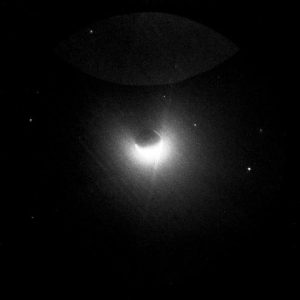
The radiation belts are not the only structures surrounding Earth. Starting from about 1,000 km, at the very edge of the inner radiation belt, and partially pushing into the outer belt, there is a cloud of charged particles called the plasmasphere. This is yet another layer of protection Earth has against space radiation. Electrons nearly at lightspeed in the outer belt move laterally along the magnetic field lines around Earth; a plasmasphere phenomenon called the plasmaspheric hiss – which is very low-frequency (VLF) electromagnetic waves – prevents them from moving down closer to Earth. This VLF hiss results in part from atmospheric lightning and in another part from ground-based transmitters communicating with submarines (Fig. 1).
The electrons in the outer belt can move into the slot region only when the Sun produces a strong solar storm or a coronal mass ejection. When they do that, the third belt appears.
The story of how these belts were discovered is equally, if not more, interesting.
In the 1950s, as ideas for space exploration were picking up, nobody knew what the environment of the part of space surrounding Earth – i.e. near space – was like. Many believed this region to be mostly a vacuum. However, scientists already knew about cosmic rays coming to Earth’s atmosphere from space, which they had studied with ground- and balloon-based instruments, and from rockets and rockoons (rockets launched from balloons at high altitudes).
In the 1950s’ US, James A. Van Allen, then chairman of the Upper Atmosphere Rocket Research Panel, launched hundreds of rockoons. He was investigating high-altitude areas near the magnetic poles. In 1953, he detected what they called ‘soft’ radiation – radiation that could be a mixture of charged particles and X-ray photons, called so because it was easily absorbed in the atmosphere – in the auroral regions above 60 km.
“The 1953 expedition yielded a remarkable new finding, namely the first direct detection of the electrons which, we surmised, were the primaries for producing auroral luminosity,” Van Allen wrote. Then, the International Geophysical Year (IGY) of 1957-1958 was announced, and on October 4, 1957, the Soviet Union launched the first artificial satellite, Sputnik 1. It showed for the first time that orbital space is safe – at least from meteoroids – for satellites.
Soviet scientists, led by Sergei Vernov at Moscow State University, weren’t much behind the Americans. For many years, even from before World War II, they had been studying cosmic rays from the ground and from balloons, and even using captured German rockets designed by Wernher von Braun. In 1956, Vernov and his staff prepared their instruments for cosmic-ray measurements in space, ready to fly on Sputnik 1. However, the launch was shrouded in secrecy, even from the eyes of Soviet scientists.
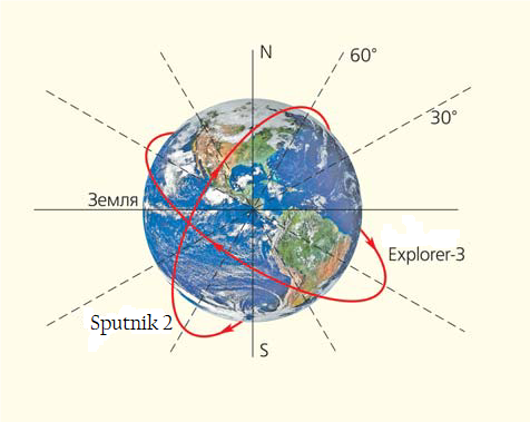
On November 3, 1957, the Soviet Union launched a more sophisticated spacecraft called Sputnik 2, which had equipment to actually measure the energy of cosmic rays. The two KS-5 counters (Kosmicheskii Schetchik in Russian) consisted of SI-17 gas discharge tubes, commonly used in high-altitude balloon studies of cosmic rays. Sputnik 2 was launched into an elliptical orbit with a perigee of 225 km, apogee of 1,671 km and a period of 103.75 minutes. It downlinked several sets of mission data: solar X-ray data, cosmic-ray counts, biometric data on the dog Laika and temperature readings.
However, the X-ray team thought their experiment had failed because the photomultiplier tubes were mostly saturated by intense radiation independent of whichever way they were pointed in space. They realised only in retrospect that these were the effects of the radiation belts. The KS-5 data, obtained between November 3 and 9, 1957, was of good quality. The increase of radiation was registered on November 7, when the satellite was at about +60° latitude over Soviet territory (Fig. 2).
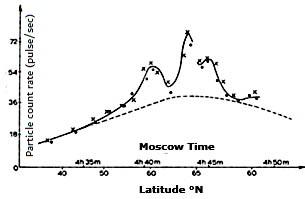
This was attributed to a weak solar flare that Vernov had reported in May 1958, in Russian and without explaining the source of the flux increase. The satellite had actually detected the space radiation, and the belts could have been called Vernov belts if not for the Cold War paranoia at that time.
The telemetry from Sputnik 2 could only be received over territorial USSR, and the spacecraft had no recording device. The apogee of the orbit (at 1,671 km) occurred over the south polar region, where it penetrated into the radiation belt, but that data was not received by Soviet stations. The Australian scientist Harry Messel recorded Sputnik 2 data when it passed over Australia, but the Soviets refused to share the interpreting codes when he asked for them. And when the Soviets asked for the data from Messer, he refused.
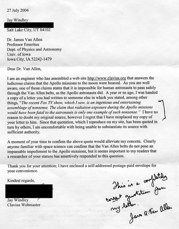
As Fred Singer, a contemporary of Van Allen’s, expressed in a letter to Alex Dressler (see appendix 1), the director of the Space Science Laboratory at the Marshall Space Flight Centre, Alabama, “When they finally asked for the copy of the recorded data, he told them to go to hell (as only Harry Messel could).”
The US launched its first satellite, Explorer 1, on January 31, 1958, with instruments to measure radiation. But the cosmic ray detector did not register any radiation in the parts where Van Allen thought it should be high, so he figured the instruments were actually saturated with particles trapped in Earth’s magnetic field. He reported this in May 1958 at the IGY lecture, attributing the particles to be of auroral origin which had somehow leaked into the equatorial region.
By March 1958, two months earlier, Explorer 3 had confirmed Explorer 1’s data, but only Sputnik 3 was able to determine the nature of these particles. This was because it also carried a scintillation counter – a 40 × 40 mm sodium iodide crystal doped with thallium. It allowed scientists to determine that particles registered in polar regions were protons of ~100 Mev energy while those in the equatorial regions were electrons with energies ~100 Kev.
Explorer 4 confirmed the existence of two distinct belts; subsequently, it turned out that Sputniks 2 and 3 had discovered the outer belt – also called the near-polar belt – while the Explorers observed the inner belt – the equatorial belt, owing to the different launch latitudes.
Apollo 11’s trans-lunar injection
After establishing that radiation belts do contain lots of highly energetic particles – protons and electrons – scientists realised they presented a problem for humans and satellites in space. The obvious solution was to limit orbits to below the inner belt, which begins at about 600 km above Earth’s surface. For example, the maximum altitude of the first human flight by Yuri Gagarin had been 327 km.
The first recommendations for dealing with the Van Allen belts on a possible mission to the Moon came in the summer of 1960, at a NASA Space Task Group meeting. Scientists suggested that a moderate amount of protection could shield a crew from the outer Van Allen belt particles. In 1962, Van Allen – believing that protons of the inner belt could seriously threaten human spaceflight missions – suggested clearing them away by setting a nuclear bomb off near the outer belt. The particles would then have the extra energy to escape Earth’s magnetic field.
The Americans conducted a series of nuclear tests in the 1960s called Operation Dominic. It included a group of atmospheric tests called the Fishbowl events, designed to understand how nuclear weapon debris would interact with Earth’s magnetic field in the event of a nuclear war. The highest of the Fishbowl events was called Starfish Prime – a 1.4-megaton nuclear bomb detonated at 400 km on July 9, 1962. However, instead of clearing the inner Van Allen belt, it actually added more radiation to it. The Soviet tests in the same year increased the intensity of the inner belt by a million-times, and also destroyed several satellites that were already there.
One of them was Telstar 1, which had been launched just the day after Starfish Prime. It relayed the first TV pictures, fax images and the first-ever transatlantic TV feeds. By October, the increased radiation from the Soviet test had burnt Telstar‘s transistors and it went out of service in 1963.
The high-energy electrons injected into the lower Van Allen belt had decayed to one-twelfth of their post-test peak intensity only by 1969.
When NASA commenced its lunar spaceflight program, its scientists already knew about the belts and their spatial and energy distribution. Apropos the energies: electrons below about 1 MeV were unlikely to be dangerous, as were protons below 10 MeV. For example, a proton with an energy of 3 MeV could penetrate about 6 mm of aluminium (a typical spacecraft material) whereas one of 100 MeV could penetrate up to 40 mm. So engineers fashioned shielding that consisted of a spacecraft hull and all the instrumentation lining the walls.
Further, knowing the belts’ absence above the poles, the altitude of the lower edge of the inner belt being ~600 km (well above the LEO) and the location of the South Atlantic anomaly, where doses are at a high 40 mrads/day at an altitude of 210 km allowed NASA to design the Apollo translunar injection (TLI) orbit in a way that the spacecraft would avoid the belts’ most dangerous parts.
Apollo 11 bypassed the inner belt and only passed through the weaker part of the outer belt (Fig. 4). According to NASA’s ‘The Apollo Spacecraft: A Chronology’, the high-altitude nuclear tests would have had a significant impact on Apollo orbits but NASA scientists had accounted for this possibility in radiation-protection planning.
Several factors worked in favour of the minimum exposure trajectory. We all know that Earth’s axis is tilted by 23.5° relative to the ecliptic plane. In 1969, the magnetic north pole was displaced from the geographical north pole by 11.4°. Therefore in 1969, the Van Allen radiation belts could have had a maximum inclination of 34.9° (23.5°+11.4°) with respect to the ecliptic (Fig. 5).
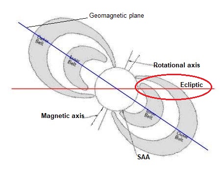
The ideal path for Apollo would’ve been through the north or south magnetic poles because that is where there are no belts. However, that would also have meant burning a lot of fuel to get into the lunar orbital plane.
The geomagnetic plane being inclined relative to the ecliptic effectively resulted in the location of the TLI point of Apollo 11 orbit being very close to the descending node of the geomagnetic plane (see Fig. 5). The elliptical nature of the transfer orbit means that its apogee will be at the same latitude in the opposite hemisphere of its perigee. So if the injection happened in the lunar orbit plane, it will end up in the same plane again when it reaches the Moon.
The Moon’s orbit is inclined by 5° relative to the ecliptic, but the Moon at the arrival of the Apollo 11 was nearly exactly in the ecliptic (at the entrance into the lunar orbit on July 19, 1969, 17:22 UTC, the Moon’s position had the ecliptic coordinates 174° geocentric longitude, 0° geocentric latitude), so that the flight path after the TLI was also nearly in the ecliptic. In fact, on the webpage ‘Apollo by the Numbers – Translunar Injection’, the inclination is specified as 31.383º.
Thus, after leaving the TLI, they travelled in the direction where the geomagnetic plane slopes away from the ecliptic. By the time Apollo 11 reached a distance of about three Earth radii, the geomagnetic axis was tilted almost exactly in the direction of the spacecraft, thus the separation between Apollo 11 and the geomagnetic plane was at its maximum.
In Fig. 4, the path is shown with 10-minute increments (red dots). It is obvious that Apollo 11’s flight path avoided areas with the highest flux. The Earth parking orbit is under the inner radiation belt; it traversed the inner zone of the outer belt in about 30 minutes and through the most energetic region in about 10 minutes. On its way back, its trajectory was optimised such that Apollo 11 would steer clear of the belts as much as possible. It approached Earth from the south and was travelling at an even greater inclination and velocity than it had been on its way to the Moon. The astronauts were inside the fringes of the radiation belts for only about 60 minutes.
Based on data from the twin Van Allen Probes NASA launched in 2012, scientists found that the inner belt is made up typically of high-energy protons and low-energy electrons. They also found that the radiation here was much weaker than what they’d assumed it to be. The most dangerous highly relativistic electrons (with energies of 0.7-1.5 MeV) couldn’t penetrate the slot region. Rather, they could but only rarely, such as when they were helped along by two severe solar storms in 2015.
NASA currently admits it overestimated the level of danger in the low and medium Earth orbits, as a result spending too much money on building heavily protected spacecraft.
However, once we’re out of near space, outer space and the lunar environment could present their own threats.
Radiation risk in outer space
Outside Earth’s magnetic field, there are about 10-20 protons per cubic cm, travelling at about 400-650 km/s. For approximately five days in each of its orbits, the Moon is inside Earth’s geomagnetic tail, where there are usually no particles from the solar wind. For another approximately five days, the Moon is in the magnetosheath, where the particle flux is reduced and the protons are slower, moving at 250-450 km/s. We were able to obtain these continuous measurements using the Solar Wind Spectrometer that the Apollo 12 left behind on the Moon.
It remains possible for astronauts to be affected by solar storms. For example, if any of them had been travelling to the Moon during the solar event of August 1972, they would have been exposed to life-threatening amounts of radiation.
The Apollo 11 crew had received 0.18 rem each on average (‘rem’ stands for ‘roentgen equivalent man’). To compare, one CT scan delivers about 1 rem. To kill an adult human, you’d have to deliver 300 rem or more in a very short span of time, but if it is spread over weeks or even days, there will be few effects. About 50 rem delivered at once will cause radiation sickness.
Even if there had been a solar storm when Neil Armstrong and Edwin “Buzz” Aldrin, Jr. were on the Moon, they could have been protected by the Apollo command module: it was built to attenuate 400 rem on the outside to less than 35 rem on the inside. Attenuation numbers are usually denoted in units of areal density, grams per sq. cm. A typical Apollo suit had a strength of 0.25 g/cm2 while the Apollo command module hull had a strength of 7-8 g/cm2. The hull of the International Space Station, to compare, has a strength of 15 g/cm2 in the specially shielded areas.
We were indeed lucky that the August 1972 event happened between the last two Apollo flights: Apollo 16 had returned in April and Apollo 17 set off to the Moon in December. No major solar particle events have occurred during the Apollo 8 or 11 missions.
Margarita Safonova is a visiting scientist at the Indian Institute of Astrophysics, Bangalore. Her broad interests are the application of gravitational lensing in astrophysics and cosmology and UV astronomy from space.