


A medic collects swab sample of a man for COVID-19 test at Narahi after a pregnant woman was found positive for coronavirus in the area, in Lucknow, Friday, May 8, 2020. Photo: PTI/Nand Kumar.
The COVID-19 pandemic has made brutally clear the need for further research into many aspects of viruses. In this article we compile data about the basic properties of the SARS-CoV-2 virus, and about how it interacts with the body (see figure below). We also discuss a number of questions about the virus, and perform ‘back-of-the-envelope’ calculations to show the insights that can be gained from knowing some key numbers and using quantitative reasoning. It is important to note that much uncertainty remains, and while ‘back-of-the-envelope’ calculations can improve our intuition through sanity checks, they cannot replace detailed epidemiological analysis.
Eight questions about SARS-CoV-2
1. How long does it take a single infected person to yield one million infected people?
If everybody continued to behave as usual, how long would it take the pandemic to spread from one person to a million infected victims? The basic reproduction number, R0, suggests each infection directly generates 2–4 more infections in the absence of countermeasures like physical distancing. Once a person is infected, it takes a period of time known as the ‘latent period’ before they are able to transmit the virus. The current best-estimate of the median latent time is ≈3 days followed by ≈4 days of close to maximal infectiousness (Li et al., 2020a; He et al., 2020).
The exact durations vary among people, and some are infectious for much longer. Using R0≈4, the number of cases will quadruple every ≈7 days or double every ≈3 days. Thousand-fold growth (going from one case to 1,000) requires 10 doublings since 210≈ 103; 3 days × 10 doublings = 30 days, or about one month. So we expect ≈1,000x growth in one month, a million-fold (106) in two months, and a billion fold (109) in three months.
Even though this calculation is highly simplified, ignoring the effects of ‘super-spreaders’, herd-immunity and incomplete testing, it emphasises the fact that viruses can spread at a bewildering pace when no countermeasures are taken. This illustrates why it is crucial to limit the spread of the virus by physical distancing measures. For fuller discussion of the meaning of R0, the latent and infectious periods, as well as various caveats, see the section on ‘Definitions and measurement methods’ below.
Also read: Moderna’s Coronavirus Vaccine Shows Promise in Data From 8 People
2. What is the effect of physical distancing?
A highly simplified quantitative example helps clarify the need for physical distancing. Suppose that you are infected and you encounter 50 people over the course of a day of working, commuting, socialising and running errands. To make the numbers round, let’s further suppose that you have a 2% chance of transmitting the virus in each of these encounters, so that you are likely to infect one new person each day. If you are infectious for 4 days, then you will infect four others on average, which is on the high end of the R0 values for SARS-CoV-2 in the absence of physical distancing. If you instead see five people each day (preferably fewer) because of physical distancing, then you will infect 0.1 people per day, or 0.4 people before you become less infectious.
The desired effect of physical distancing is to make each current infection produce <1 new infections. An effective reproduction number (Re) smaller than one will ensure the number of infections eventually dwindles. It is critically important to quickly achieve Re < 1, which is substantially more achievable than pushing Re to near zero through public health measures.
3. Why was the initial quarantine period two weeks?
The period of time from infection to symptoms is termed the incubation period. The median SARS-CoV-2 incubation period is estimated to be roughly 5 days (Lauer et al., 2020). Yet there is much person-to-person variation. Approximately 99% of those showing symptoms will show them before day 14, which explains the two-week confinement period. Importantly, this analysis neglects infected people who never show symptoms. Since asymptomatic people are not usually tested, it is still not clear how many such cases there are or how long asymptomatic people remain infectious for.
4. How do N95 masks block SARS-CoV-2?
N95 masks are designed to remove more than 95% of all particles that are at least 0.3 microns (µm) in diameter. In fact, measurements of the particle filtration efficiency of N95 masks show that they are capable of filtering ≈99.8% of particles with a diameter of ≈0.1 μm (Rengasamy et al., 2017). SARS-CoV-2 is an enveloped virus ≈0.1 μm in diameter, so N95 masks are capable of filtering most free virions, but they do more than that. How so?
Viruses are often transmitted through respiratory droplets produced by coughing and sneezing. Respiratory droplets are usually divided into two size bins, large droplets (>5 μm in diameter) that fall rapidly to the ground and are thus transmitted only over short distances, and small droplets (≤5 μm in diameter). Small droplets can evaporate into ‘droplet nuclei’, remain suspended in air for significant periods of time and could be inhaled. Some viruses, such as measles, can be transmitted by droplet nuclei (Tellier et al., 2019).
Larger droplets are also known to transmit viruses, usually by settling onto surfaces that are touched and transported by hands onto mucosal membranes such as the eyes, nose and mouth (CDC, 2020). The characteristic diameter of large droplets produced by sneezing is ~100 μm (Han et al., 2013), while the diameter of droplet nuclei produced by coughing is on the order of ~1 μm (Yang et al., 2007). At present, it is unclear whether surfaces or air are the dominant mode of SARS-CoV-2 transmission, but N95 masks should provide some protection against both (Jefferson et al., 2009; Leung et al., 2020).
Also read: The Fluid Dynamics of How the Novel Coronavirus Moves Around
5. How similar is SARS-CoV-2 to the common cold and flu viruses?
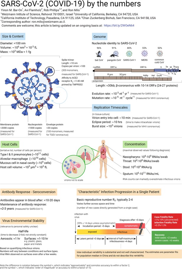
SARS-CoV-2 is a beta-coronavirus whose genome is a single ≈30 kb strand of RNA[footnote]’kb’ stands for kilobase, or 1,000 bases[/footnote]. The flu is caused by an entirely different family of RNA viruses called influenza viruses. Flu viruses have smaller genomes (≈14 kb) encoded in eight distinct strands of RNA, and they infect human cells in a different manner than coronaviruses.
The ‘common cold’ is caused by a variety of viruses, including some coronaviruses and rhinoviruses. Cold-causing coronaviruses (e.g. OC43 and 229E strains) are quite similar to SARS-CoV-2 in genome length (within 10%) and gene content, but different from SARS-CoV-2 in sequence (≈50% nucleotide identity) and infection severity. One interesting facet of coronaviruses is that they have the largest genomes of any known RNA viruses (≈30 kb). These large genomes led researchers to suspect the presence of a ‘proofreading mechanism’ to reduce the mutation rate and stabilise the genome.
Indeed, coronaviruses have a proofreading exonuclease called ExoN, which explains their low mutation rates (~10–6 per site per cycle) in comparison to influenza (≈3 × 10⁻⁵ per site per cycle; Sanjuán et al., 2010). This relatively low mutation rate will be of interest for future studies predicting the speed with which coronaviruses can evade our immunisation efforts.
Also read: How Does Remdesivir Work Against the Novel Coronavirus?
6. How much is known about the SARS-CoV-2 genome and proteome?
SARS-CoV-2 has a single-stranded positive-sense RNA genome that codes for 10 genes ultimately producing 26 proteins according to an NCBI annotation (NC_045512). How is it that 10 genes code for >20 proteins? One long gene, orf1ab, encodes a polyprotein that is cleaved into 16 proteins by proteases that are themselves part of the polyprotein. In addition to proteases, the polyprotein encodes an RNA polymerase and associated factors to copy the genome, a proofreading exonuclease, and several other non-structural proteins.
The remaining genes predominantly code for structural components of the virus: i) the spike protein which binds the cognate receptor on a human or animal cell; ii) a nucleoprotein that packages the genome; iii) two membrane-bound proteins. Though much current work is centred on understanding the role of ‘accessory’ proteins in the viral life cycle, we estimate that it is currently possible to ascribe clear biochemical or structural functions to only about half of SARS-CoV-2 gene products.
7. What can we learn from the mutation rate of the virus?
Studying viral evolution, researchers commonly use two measures describing the rate of genomic change. The first is the evolutionary rate, which is defined as the average number of substitutions that become fixed per year in strains of the virus, given in units of mutations per site per year. The second is the mutation rate, which is the number of substitutions per site per replication cycle. How can we relate these two values?
Consider a single site at the end of a year. The only measurement of a mutation rate in a β-coronavirus suggests that this site will accumulate ~10–6 mutations in each round of replication. Each replication cycle takes ~10 hr, and so there are 103 cycles/year. Multiplying the mutation rate by the number of replications, assuming neutrality and neglecting the effects of evolutionary selection, we arrive at 10–3 mutations per site per year, consistent with the evolutionary rate inferred from sequenced coronavirus genomes.
As our estimate is consistent with the measured rate, we infer that the virus undergoes near-continuous replication in the wild, constantly generating new mutations that accumulate over the course of the year. Using our knowledge of the mutation rate, we can also draw inferences about single infections. For example, since the mutation rate is ~10–6 mutations/site/cycle and an mL of sputum might contain upwards of 107 viral RNAs, we infer that every site is mutated more than once in such samples.
8. How stable and infectious is the virion on surfaces?
To understand how SARS-CoV-2 can be transmitted, it is vitally important to characterise the stability of infectious virions on different types of surfaces like cardboard, plastics, and various metals. This is a very active area of current research. However, there are significant caveats associated with viral stability measurements.
The measured stability depends on the quantity measured, for example, one can measure either infectious virions or viral RNA copies. The number of infectious virions is typically much lower than inferred from measurements of the viral genome (Woelfel et al., 2020). SARS-CoV-2 RNA has been detected on various surfaces several weeks after they were last touched (Moriarty et al., 2020), but infectiousness appears to degrade more quickly than RNA. When researchers measured the stability of infectious virions on surfaces, the numbers depended greatly on the type of surface and the medium carrying the virus, with the stability on plastic being much greater than on copper or steel, for example.
Viral stability is also known to depend strongly on temperature and humidity (Chin et al., 2020). Therefore calculating the probability of human infection from exposure to contaminated surfaces is a complex task for which sufficient data is not yet available. As such, caution and protective measures should be taken. To gain some intuition for the importance of surface transmission, we consider an undiagnosed infectious person who touches surfaces tens of times during their infectious period. Prior to lockdown, these public surfaces will subsequently be touched by hundreds of other people. From the basic reproduction number R0 ≈ 2–4 we can infer that not everyone touching those surfaces will be infected.
More detailed bounds on the risk of infection from touching surfaces urgently awaits study.
Also read: New Virus Lasts Hours on Surfaces, in Air but Proximity to Patients Is Riskier
Definitions and measurement methods
1. What are the meanings of R0, ‘latent period’ and ‘infectious period’?
The basic reproduction number, R0, estimates the average number of new infections directly generated by a single infectious person. The ‘0’ subscript connotes that this refers to early stages of an epidemic, when everyone in the region is susceptible (that is, there is no immunity) and no countermeasures have been taken. As geography and culture affect how many people we encounter daily, how much we touch them and share food with them, estimates of R0 can vary between locales.
Moreover, because R0 is defined in the absence of countermeasures and immunity, we are usually only able to assess the effective R (Re). At the beginning of an epidemic, before any countermeasures, Re ≈ R0. Several days pass before a newly-infected person becomes infectious themselves. This ‘latent period’ is typically followed by several days of infectivity called the ‘infectious period’.
It is important to understand that reported values for all these parameters are population averages inferred from epidemiological models fit to counts of infected, symptomatic, and dying patients. Because testing is always incomplete and model fitting is imperfect, and data will vary between different locations, there is substantial uncertainty associated with reported values. Moreover, these median or average best-fit values do not describe person-to-person variation.
For example, viral RNA was detectable in patients with moderate symptoms for more than one week after the onset of symptoms, and more than two weeks in patients with severe symptoms (ECDC, 2020). Though detectable RNA is not the same as active virus, this evidence calls for caution in using uncertain, average parameters to describe a pandemic. Why have detailed distributions of these parameters across people not been published?
Direct measurement of latent and infectious periods at the individual level is extremely challenging, as accurately identifying the precise time of infection is usually very difficult.
Also read: Our COVID-19 Strategy Depends on the R0 Number. Do We Know the R0 Number?
2. What is the difference between measurements of viral RNA and infectious viruses?
Diagnosis and quantification of viruses utilises several different methodologies. One common approach is to quantify the amount of viral RNA in an environmental (e.g. surface) or clinical (e.g. sputum) sample via quantitative reverse-transcription polymerase chain reaction (RT-qPCR). This method measures the number of copies of viral RNA in a sample. The presence of viral RNA does not necessarily imply the presence of infectious virions. Virions could be defective (e.g., by mutation) or might have been deactivated by environmental conditions.
To assess the concentration of infectious viruses, researchers typically measure the ‘50% tissue-culture infectious dose’ (TCID50). Measuring TCID50 involves infecting replicate cultures of susceptible cells with dilutions of the virus and noting the dilution at which half the replicate dishes become infected. Viral counts reported by TCID50 tend to be much lower than RT-qPCR measurements, which could be one reason why studies relying on RNA measurements (Moriarty et al., 2020) report the persistence of viral RNA on surfaces for much longer times than studies relying on TCID50 (van Doremalen et al., 2020).
It is important to keep this caveat in mind when interpreting data about viral loads, for example a report measuring viral RNA in patient stool samples for several days after recovery (Wu et al., 2020a). Nevertheless, for many viruses even a small dose of virions can lead to infection. For the common cold, for example, ~0.1 TCID50 are sufficient to infect half of the people exposed (Couch et al., 1966).
3. What is the difference between the case fatality rate and the infection fatality rate?
Global statistics on new infections and fatalities are pouring in from many countries, providing somewhat different views on the severity and progression of the pandemic. Assessing the severity of the pandemic is critical for policymaking and thus much effort has been put into quantifying key measures of its progression.
The most common measure for the severity of a disease is the fatality rate. One commonly reported measure is the case fatality rate (CFR), which is the proportion of fatalities out of total diagnosed cases. The CFR reported in different countries varies significantly, from 1% to about 15%. Several key factors affect the CFR. First, demographic parameters and practices associated with increased or decreased risk differ greatly across societies. For example, the prevalence of smoking, the average age of the population, and the capacity of the healthcare system.
Indeed, the majority of people dying from SARS-CoV-2 have a preexisting condition such as cardiovascular disease or smoking (The Novel Coronavirus Pneumonia Emergency Response Epidemiology Team, 2020). There is also potential for bias in estimating the CFR. For example, a tendency to identify more severe cases (selection bias) will tend to overestimate the CFR. On the other hand, there is usually a delay between the onset of symptoms and death, which can lead to an underestimate of the CFR early in the progression of an epidemic. We report the uncorrected CFR values, and thus these caveats should be borne in mind.
Even when correcting for these factors, the CFR does not give a complete picture as many cases with mild or no symptoms are not tested. Thus, the CFR will tend to overestimate the rate of fatalities per infected person, termed the infection fatality rate (IFR). Estimating the total number of infected people is usually accomplished by testing a random sample for anti-viral antibodies, whose presence indicates that the patient was previously infected.
At the time of writing, such assays are not widely available, and so researchers resort to surrogate datasets generated by testing of foreign citizens returning home from infected countries (Verity et al., 2020; Nishiura et al., 2020), large-scale semi-random testing in countries such as Iceland, near complete testing of passengers on the Diamond Princess ship (Russell et al., 2020), or epidemiological models estimating the number of undocumented cases (Li et al., 2020a; Mizumoto et al., 2020). These methods have their own caveats and uncertainties associated with them, and it is not entirely clear how representative they are but they do provide a first glimpse of the true severity of the disease.
Also read: What We Know About Whom COVID-19 Kills
4. What is the burst size and the replication time of the virus?
Two important characteristics of the viral life cycle are the time it takes them to produce new infectious progeny, and the number of progeny each infected cell produces. The yield of new virions per infected cell is more clearly defined in lytic viruses, such as those infecting bacteria (bacteriophages), as viruses replicate within the cell and subsequently lyse the cell to release a ‘burst’ of progeny. This measure is usually termed ‘burst size’.
SARS-CoV-2 does not release its progeny by lysing the cell, but rather by continuous budding (Park et al., 2020b). Even though there is no ‘burst’, we can still estimate the average number of virions produced by a single infected cell. Measuring the time to complete a replication cycle or the burst size in vivo is very challenging, and thus researchers usually resort to measuring these values in tissue-culture.
There are various ways to estimate these quantities, but a common and simple one is using ‘one-step’ growth dynamics. The key principle of this method is to ensure that only a single replication cycle occurs. This is typically achieved by infecting the cells with a large number of virions, such that every cell gets infected, thus leaving no opportunity for secondary infections.
Assuming entry of the virus to the cells is rapid (we estimate 10 min for SARS-CoV-2), the time it takes to produce progeny can be estimated by quantifying the lag between inoculation and the appearance of new intracellular virions, also known as the ‘eclipse period’. This eclipse period does not account for the time it takes to release new virions from the cell. The time from cell entry until the appearance of the first extracellular viruses, known as the ‘latent period’ (not to be confused with the epidemiological latent period), estimates the duration of the full replication cycle. The burst size can be estimated by waiting until virion production saturates, and then dividing the total virion yield by the number of cells infected.
While both the time to complete a replication cycle and the burst size may vary significantly in an animal host due to factors including the type of cell infected or the action of the immune system, these numbers provide us with an approximate quantitative view of the viral life-cycle at the cellular level.
5. Are people usually diagnosed before or after they are contagious?
Our personal experience with infectious diseases leaves us with the intuition that we are contagious when we have symptoms. For the seasonal flu, for example, most transmissions indeed occur after a person has developed symptoms (Ip et al., 2017). For SARS-CoV-2, in contrast, it is common to be contagious before symptoms. The SARS-CoV-2 incubation period is about 5 days, while peak infectiousness begins two days before symptoms reveal themselves. As a result, a large fraction of infections occur pre-symptomatically, that is, without the infectious person realising they have the disease (Ferretti et al., 2020; He et al., 2020).
With testing capacity under strain, diagnosis typically occurs ≈5 days after symptom onset, or ≈10 days after infection. By that time, most people have already passed peak infectiousness. In order to effectively slow the growth of the pandemic, it is important to detect infections as early as possible and quarantine those who test positive. In the case of SARS-CoV-2 this means detection before symptoms because there is strong evidence of significant pre-symptomatic transmission. Finally, the situation is further complicated by a large fraction of asymptomatic cases, that is cases in which the infected person never develops noticeable symptoms. This fraction is more than half of children and young adults (Davies et al., 2020).
Leading modelling efforts assume that asymptomatic infections are anywhere between 10–80% as contagious as symptomatic ones (Ferretti et al., 2020; Davies et al., 2020). This wide range reflects a crucial gap in our understanding of SARS-CoV-2 transmission: great uncertainty about the magnitude of asymptomatic transmission.
Yinon M Bar-On and Ron Milo are with the department of plant and environmental sciences, Weizmann Institute of Science, Israel. Avi Flamholz is with the department of molecular and cell biology, University of California, Berkeley. Rob Phillips is with the department of physics, department of applied physics, and the division of biology and biological engineering, California Institute of Technology, Pasadena, and the Chan Zuckerberg Biohub, San Francisco.
This article was originally published on eLife and has been republished here under a Creative Commons Attribution license.